Obtaining R
Download R from the main project at http://www.r-project.org/
Invoking and Quitting
The command for starting R is simply R. Once R is started, it may be stopped via the quit() function.
$ R

R : Copyright 2004, The R Foundation for Statistical Computing
Version 2.0.1  (2004-11-15), ISBN 3-900051-07-0

R is free software and comes with ABSOLUTELY NO WARRANTY.
You are welcome to redistribute it under certain conditions.
Type 'license()' or 'licence()' for distribution details.

R is a collaborative project with many contributors.
Type 'contributors()' for more information and
'citation()' on how to cite R or R packages in publications.

Type 'demo()' for some demos, 'help()' for on-line help, or
'help.start()' for a HTML browser interface to help.
Type 'q()' to quit R.

> quit()
Save workspace image? [y/n/c]: n
$
Data and Variables
There are two straightforward ways to enter a simple list of data to use in R. Both make use of the assignment operator <- which assigns a value (on the right) to a variable (pointed to on the left). The first is to use the concatenate function c() to create a list (a vector in math terms) of values. The second is to use the scan() function to read in raw space-separated data.
Note: While the <- operator is traditional, the = operator also functions for assignment. I tend to use the left arrow in most of my examples, but I do lapse occasionally into the other equally valid notation.
> a <- c( 1, 2, 3, 4 )
> a
[1] 1 2 3 4
> b <- scan()
1: 1 2
3: 3 4
5:
Read 4 items
> b
[1] 1 2 3 4
Use ls() and rm() to list or remove variables that you have previously created. If there are no variables defined, ls() may report "character(0)".
> a <- c( 1, 2, 3, 4 )
> ls()
[1] "a"
> rm( a )
> ls()
character(0)
Simple descriptive statistics
The most commonly-used descriptive statistics are returned easily via functions like mean(), sd(), etc.
> a <- c( 1, 2, 4, 8 )
> mean( a )                           # sample mean
[1] 3.75
> median( a )                         # sample median
[1] 3
> var( a )                            # sample variance
[1] 9.583333
> sd( a )                             # sample standard deviation
[1] 3.095696
> quantile( a )                       # quartiles (note the name of the function is quantile, not quartile)
  0%  25%  50%  75% 100%
1.00 1.75 3.00 5.00 8.00
> quantile( a, type=2 )                # also quartiles but handles the "in between" cases like Sullivan
  0%  25%  50%  75% 100%
 1.0  1.5  3.0  6.0  8.0
> quantile( a, type=6 )                # also quartiles -- method used by Minitab and SPSS
  0%  25%  50%  75% 100%
1.00 1.25 3.00 7.00 8.00
> length( a )                         # number of items in the vector a
[1] 4
> max( a )                            # maximum value
[1] 8
> min( a )                            # minimum value
[1] 1
> fivenum( a )                        # five number summary
[1] 1.0 1.5 3.0 6.0 8.0
Statistical plots
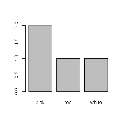
Table, bar chart, and pie chart
Perhaps the simplest way to arrange data is in a table. The table() function of R creates tables. Notice that the next example also shows how to read categorical data in using the scan() function (by specifying that the data to be read will be character data rather than the default—numeric data).
> colors <- scan( what="character" )
1: red pink
3: pink white
5:
Read 4 items
> table( colors )
colors
pink red white
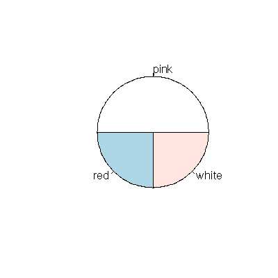
2 1 1To plot the same table as a bar chart, pass the output of the table to the barplot() function:
> barplot( table( colors ))
and as a pie chart
> pie( table( colors ))
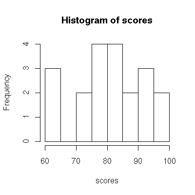
Stem-leaf plot and histogram
Use stem() to generate a stem-leaf plot, and hist() to generate a histogram.
> scores <- scan()
1: 98.0 96.0 95.0 93.0 92.0
6: 89.0 86.0 83.0 82.0 81.0 81.0 80.0
13: 79.0 79.0 77.0 74.0 73.0
18: 62.0 60.0 60.0
21:
Read 20 items
> stem( scores )

  The decimal point is 1 digit(s) to the right of the |

  6 | 002
  7 | 34799
  8 | 0112369
  9 | 23568

> hist( scores )                      # generates a histogram
A word of caution is in order. The stem() command in R will attempt to make plots that are of a "nice" size, and it may create the stems differently than you would. If you don’t read the plot carefully, you can make a mistake. Consider for example:
> scores <- scan()
1: 92 88 87 86 86 77 74 71 62 60 55 31
11:
Read 10 items
> stem( scores )

  The decimal point is 1 digit(s) to the right of the |

  2 | 1
  4 | 5
  6 | 02147
  8 | 66782
Notice, in the plot above, that the value 92 is lumped in with the 80s, coming after 80+8 as 80+12. The 55 is also very unintuitively lumped into the 40s and the 31 is in the 20s. You can adjust the scale of the plot to give it an appearance more sensible to us. Is this case, if we ask for a plot 2 times as long as normal, the appearance is better:
> stem( scores, scale=2 )
The decimal point is 1 digit(s) to the right of the |
3 | 1
4 |
5 | 5
6 | 02
7 | 147
8 | 6678
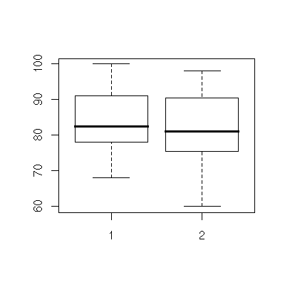
9 | 2Box plots
Use boxplot() to draw single box plots, or multiple boxplots together.
> test1 <- scan()
1: 100.0
2: 92.0 92.0 91.0 91.0 91.0 90.0
8: 86.0 86.0 83.0 82.0 81.0 80.0 80.0
15: 78.0 78.0 77.0 75.0 74.0
20: 68.0
21:
Read 20 items
> test2 <- scan()
1: 98.0 96.0 95.0 93.0 92.0
6: 89.0 86.0 83.0 82.0 81.0 81.0 80.0
13: 79.0 79.0 77.0 74.0 73.0
18: 62.0 60.0 60.0
21:
Read 20 items
> boxplot( test1 )
> boxplot( test1, test2 )
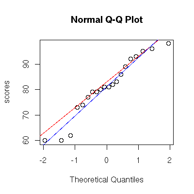
Normal probability plot
Use qqnorm() to generate a normal probability plot, and qqline() to add a line to an existing plot. If you prefer your normal reference line to be computed the same way as SPSS, use the abline() function to add the line by hand.
> scores <- scan()
1: 98.0 96.0 95.0 93.0 92.0
6: 89.0 86.0 83.0 82.0 81.0 81.0 80.0
13: 79.0 79.0 77.0 74.0 73.0
18: 62.0 60.0 60.0
21:
Read 20 items
> qqnorm( scores, ylab="scores" )
> qqline( scores, col="red" )                     # adds line through 1st and 3rd quartile
> abline( mean(scores), sd(scores), col="blue" )  # adds line through theoretical normal
Correlation and regression
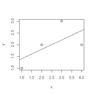
Scatter plot
The plot() function generates scatter plots. The abline() function adds a line to an existing scatter plot
and is particularly useful when fed via the linear model function lm() (to add a regression line).
> x <- c( 1,2,3,4 )
> y <- c( 1,2,3,2 )
> plot(x,y)
> abline( lm( y ~ x ))
Correlation and the regression line coefficients
For the data below, the correlation coefficient is returned by cor() and a line of best fit is calculated via lm().
> x <- c( 1,2,3,4 )
> y <- c( 1,2,3,2 )
> cor( x, y )
[1] 0.6324555
> lm( y ~ x )

Call:
lm(formula = y ~ x)

Coefficients:
(Intercept)            x
        1.0          0.4
The binomial distribution
When computing the probability of a single outcome (as opposed to a range of values) it is most convenient to use the density function dbinom(x,n,prob), which returns P( X = x ). For example, what is the probability that we observe exactly 3 ones if we toss 10 dice?
> dbinom( 3, 10, 1/6 )
[1] 0.1550454
We can also compute the combined probability of many outcomes together by summing. For example, what is the probability we observe at most 3 ones if we toss 10 dice (i.e. 0, 1, 2, or 3 ones)?
> sum( dbinom( 0:3, 10, 1/6 ))
[1] 0.9302722
Although summing works, R contains a function computing the area in a tail under the distribution function, the pbinom(x,n,prob) function. In practical terms, it is the function that takes an x-value (number of observations seen), and n-value (number of trials in the experiment), and a prob-value (probability of success) and returns P( X ≤ x ). So the probability of seeing at most 3 ones on a toss of 10 dice is:
> pbinom( 3, 10, 1/6 )
[1] 0.9302722
The qbinom(p,n,prob) function calculates essentially the inverse of the inverse of the pbinom function, the binomial quantile function. Given a probability p, it returns an x-value with P( X<x ) ≤ p. Consider an example where probability of success is 0.27 and we do 65 trials. We want to know the smallest number of successes we could expect to see "most" of the time, say 99% of the time. Another way to say this is that we want P( X<x ) = 0.01 or smaller and we’d like to know x.
> qbinom( 0.01, 65, 0.27 )
[1] 10
According to this, if we have 65 trials, each with a probability of success at 0.27 we are 99% certain of observing 10 or more successes.
The normal distribution and z-scores
The pnorm() function calculates areas under the normal probability distribution function. In practical terms, it is the function that takes z-values and returns p-values.
> pnorm( -1.645 )
[1] 0.04998491
> pnorm(1) - pnorm(-1)              # about 68% of data is within 1 std deviation of zero
[1] 0.6826895
The qnorm() function is the inverse of the pnorm() function. When given p-values, it returns z-values.
> qnorm( 0.04998491 )
[1] -1.645
> qnorm( 0.5 )
[1] 0
Plots of the normal distribution
We can get a picture of the normal distribution function. This is the curve we usually draw; the areas under it represent probabilities.
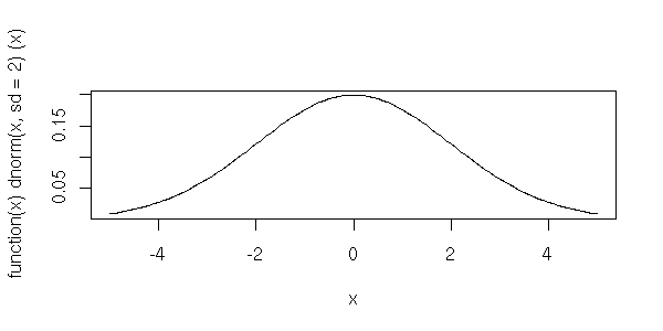
> plot( dnorm, -5, 5)Other normal distributions (that require arguments) can be plotted with the help of "anonymous functions", like the following distribution which has a standard deviation of 2.
> plot( function(x) dnorm(x,sd=2), -5, 5)
The Student’s t distribution
The pt() function calculates areas under the t distribution function. In practical terms, it is the function that takes t-values (and the number of degrees of freedom) and returns p-values.
> pt( -1, df=15 )                   # t=-1, df=15
[1] 0.1665851
The qt() function is the inverse of the pt() function. When given p-values (and degrees of freedom), it returns t-values.
> qt( 0.1665851, df=15 )            # p=0.1665851, df=15
-0.9999999
T tests
R can perform 1 variable and 2 variable t tests. Alternative hypotheses can be "less", "greater", and "two.sided". For example, we can solve this exercise from the book (Section 10.3 #23): The mean waiting time at a restaurant is 84.3 seconds. A manager devises a new system and randomly measures some wait times, 108.5, 67.4, 58.0, 75.9, 65.1, 80.4, 95.5, 86.3, 70.9, 72. Is there evidence that the new method works? Use alpha=0.01.
> wait = c( 108.5, 67.4, 58.0, 75.9, 65.1, 80.4, 95.5, 86.3, 70.9, 72 )

> boxplot( wait )                            # check normality conditions

> qqnorm( wait, ylab="wait times" )
> qqline( wait )                             # another normality check

> t.test( wait, alternative="less", mu=84.3 )

        One Sample t-test

data:  wait
t = -1.3102, df = 9, p-value = 0.1113
alternative hypothesis: true mean is less than 84.3
95 percent confidence interval:
     -Inf 86.81408
sample estimates:
mean of x
       78
With a p-value much greater than the stated alpha=0.01 we fail to reject.
Plots of the t distribution
We can get a picture of the t distribution function. This is the curve we usually draw; the areas under it represent probabilities. For example, this is the t distribution with 3 degrees of freedom.
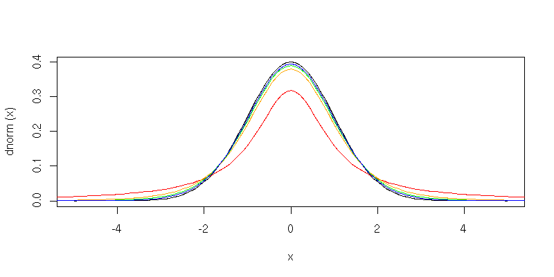
> plot( function(x) dt(x,df=3), -5, 5 )To see that the t distribution becomes more normal as the number of degrees of freedom increases, we could plot several together.
> plot( dnorm, -5, 5 )
> curve( dt(x,df=1), add=TRUE, col="red" )
> curve( dt(x,df=5), add=TRUE, col="orange" )
> curve( dt(x,df=10), add=TRUE, col="green" )
> curve( dt(x,df=20), add=TRUE, col="blue" )
The Chi Squared distribution
The pchisq() function calculates the chi squared distribution function. It is the function that takes chi-squared values (and the number of degrees of freedom) and returns p-values.
> pchisq( 11.071, 5 )                   # chi^2=11.071, df=5
[1] 0.9500097
The qchisq() function is the inverse of the pchisq() function. When given p-values (and degrees of freedom), it returns chi-squared values.
> qchisq( .95, 5 )                     # p=0.96, df=5
[1] 11.07050
Chi square tests
R can perform chi square tests. For example, we can solve this exercise from the book (section 12.1 #11): A bag of plain M&Ms should contain 13% brown, 14% yellow, 13% red, 24% blue, 20% orange, and 16% green candies. A randomly selected bag contained 61 brown, 64 yellow, 54 red, 61 blue, 96 orange, 64 green. Test whether the bag follows the stated distribution.
> observed = c( 61, 64, 54, 61, 96, 64 )
> probs = c( .13, .14, .13, .24, .20, .16 )
> chisq.test( observed, p=probs )

        Chi-squared test for given probabilities

data:  observed
X-squared = 18.7379, df = 5, p-value = 0.002151
If our significance level was alpha=0.05, we can see to reject.
Test of proportion
R can do hypothesis tests for proportions, although it uses the chi-squared distribution for the calculation. Alternative hypotheses can be "less", "greater", or "two.sided". For example, we can work this exercise from the book (Section 12.1 #23): According to the Census Bureau, 7.1% of babies with non-smoking mothers have low birth weight. To see if mothers from 35 to 39 had had more low weight babies, a random sample measured 15 low weight babies out of 160 births. Test using alpha = 0.05.
> prop.test( 15,160, p=0.071, alternative="greater", correct=FALSE )    # compute without correction for continuity

        1-sample proportions test without continuity correction

data:  15 out of 160, null probability 0.071
X-squared = 1.2555, df = 1, p-value = 0.1313
alternative hypothesis: true p is greater than 0.071
95 percent confidence interval:
 0.06231625 1.00000000
sample estimates:
      p
0.09375
Since the p-value is larger than 0.05, we fail to reject.
Making a plot ready to print
All of the plots that R generates can be saved into files. To create a PDF of a graphic, use the pdf() function before your plot. To create a PNG (portable network graphic), use the png() function before your plot. In either case, use dev.off() when finished to close the file.
> scores <- scan()
1: 98.0 96.0 95.0 93.0 92.0
6: 89.0 86.0 83.0 82.0 81.0 81.0 80.0
13: 79.0 79.0 77.0 74.0 73.0
18: 62.0 60.0 60.0
21:
Read 20 items
> pdf( file="scores-box.pdf", width=4, height=4 )    # 4 inches by 4 inches
> boxplot( scores )
> dev.off()
null device
          1
> png( file="scores-box.png", width=400, height=400 ) # 400 pixels by 400 pixels
> boxplot( scores )
> dev.off()
null device
          1
Embedding fonts in a PDF file
In some situations, you may wish to have R embed its fonts into PDF files you create (particularly if you substitute different fonts for the standard font set). You can add them using the embedFonts() function on a file you’ve already created to run ghostscript and process it.
> embedFonts(file="scores-box.pdf", outfile = "scores-box-new.pdf", options="-dPDFSETTINGS=/printer")Defining a function
> f <- function(x,y) {
+ x*y;
+ }
> f(2,3)
[1] 6
Combinations and Permutations
I don’t know of any capacity for computing combinations and permutations in R, but it is easy to add these by defining functions. We’ll create comb(n,k) and perm(n,k) for this.
> comb = function(n,k) {
  ans = 1;
  if( k>0 ) for (i in 1:k ) {
    ans = ans*n/i;
    n = n-1;
  }
  ans
}
and
> perm = function(n,k) {
  ans = 1;
  if( k>0 ) for (i in 1:k ) {
    ans = ans*n;
    n = n-1;
  }
  ans
}
Then it is a simple matter of using these functions in calculations.
> perm(10,3)
[1] 720
> comb(10,3)
[1] 120
Generating example data
Random numbers
Uniformly distributed random numbers (i.e. the kind of random numbers you get from rolling a fair die) are generated with the runif() function. By default, the random numbers come from the interval (0,1) but that may be adjusted via arguments. One argument is always required: a count of random numbers to produce.
> runif(1)
[1] 0.04546021
> runif(5)
[1] 0.469201797 0.937904294 0.921588341 0.004126997 0.622614311
> runif(1,max=6)
[1] 5.399647
For simple "die rolling," i.e. random integer numbers, this function may be convenient:
> roll = function( rolls=1, sides=6 ) {
  floor(runif( rolls, max=sides ))+1
}
And here are some examples:
> roll()              # roll a 6-sided die (default action with no arguments)
[1] 2
> roll(3)             # roll 3 dice
[1] 2 5 1
> roll(sides=10)      # roll a 10-sided die
[1] 7
> roll(3, 10)         # roll 3 10-sided dice
[1] 4 7 6
The normal approximation to the binomial distribution
The distributions that R knows about can be used to generate example data (or samples). Say we want to conduct a binomial experiment where we roll 5 dice and count the number of ones. We’d like to get an idea of the shape of this distribution, so we’ll repeat the experiment 100 times and see what the outcomes are. We use rbinom(n,k,p), which generates random numbers according to the binomial distribution.
> a = rbinom(100, 5, 1/6)
> stem(a)

  The decimal point is at the |

  0 | 0000000000000000000000000000000000000000000
  0 |
  1 | 00000000000000000000000000000000000
  1 |
  2 | 0000000000000000
  2 |
  3 | 000000
This is decidedly non-normal, but we can verify that things are different if the number of dice is different. Verify that the number of ones appearing on a roll of 72 dice is approximately normally distributed with a mean of 12 and a standard deviation of 3.162278.
> a = rbinom(100,72,1/6)
> stem(a)

  The decimal point is at the |

   4 | 0
   6 | 0000
   8 | 00000000000000
  10 | 000000000000000000
  12 | 00000000000000000000000000
  14 | 0000000000000000000
  16 | 00000000000000
  18 | 00
  20 | 00

> mean(a)
[1] 12.5
> sd(a)
[1] 3.131786
Normal data
We can generate random numbers based on the normal distribution just as easily. For example, we’d like a random sample of 20 items from a normally distributed population that has mean 50 and standard deviation about 8.
> rnorm(20, mean=50, sd=8)
 [1] 46.76492 56.54318 38.80065 40.58243 46.18913 31.09232 29.51878 38.60033
 [9] 51.89929 45.93668 60.25701 49.84637 43.12018 46.71614 42.53040 53.01289
[17] 61.80566 62.21275 48.14231 36.18348
Perhaps we would prefer integers for our example data set.
> a = round( rnorm(20, mean=50, sd=8))
> mean(a)
[1] 50.95
> sd(a)
[1] 6.801509
> stem(a)
Modeling the central limit theorem with random numbers
I have an entire page devoted to modeling the central limit theorem using R’s built-in random number generators. Check it out at:
ModelCLTmean.html Central limit theorem for the sample mean.
ModelCLTprop.html Central limit theorem for the sample proportion.
Samples and the central limit theorem
From the book, we learn that human pregnancies last an average of 266 days and are approximately normally distributed with a standard deviation of 16. We can simulate a data set of 10,000 pregnancies using random numbers.
> a = round( rnorm(10000, mean=266, sd=16 ))Now that we have a simulated population, we can use the sample() function to take random samples from it. For example, if we would like a random sample of size 4:
> sample(a,4)
[1] 277 260 276 293
> sample(a,4)
[1] 272 282 301 266
> sample(a,4)
[1] 258 256 245 274
Or we might compute the mean of a sample of size 4:
> mean( sample(a,4))
[1] 266.75
The central limit theorem tells us that the sampling distribution of the mean will have the same center as the parent population, but a smaller standard deviation. We can verify the sampling distribution of the mean (for samples of size 4) looks normal also with standard deviation of 16/sqrt(4). Here we use replicate() to find the means of 100 different samples of size 4; then we compute the mean and standard deviation. Note how close the results are to 266 and 8.
> b = replicate(100, mean(sample(a,4)))
> b
  [1] 268.50 271.00 272.25 278.00 268.75 264.00 253.00 276.75 244.50 272.00
 [11] 270.25 284.75 256.50 276.00 277.00 271.50 271.75 272.00 269.25 269.25
 [21] 259.25 275.75 262.00 270.25 261.00 270.00 272.25 267.75 279.00 264.50
 [31] 269.50 271.00 274.00 274.50 261.75 264.50 261.00 258.25 262.25 275.25
 [41] 259.50 271.50 256.75 276.00 254.50 271.75 274.50 272.25 262.00 281.25
 [51] 272.75 262.25 270.75 271.25 268.00 262.75 274.75 254.00 277.75 265.50
 [61] 271.25 268.75 268.50 274.75 259.50 255.00 259.00 252.00 266.00 264.75
 [71] 267.75 263.25 266.25 263.25 269.50 252.50 254.75 278.00 267.00 263.75
 [81] 268.25 275.50 261.75 260.25 267.75 268.50 271.25 274.25 278.25 270.50
 [91] 270.00 270.25 251.75 272.00 266.00 267.75 268.00 270.50 260.75 248.75
> mean(b)
[1] 267.28
> sd(b)
[1] 7.643929