Plotting Functions

If a graph is too tall an needs to be truncated, you can also specify a range. Contrast the following 2 plots:

Since Octave is not a computer algebra system, the way it handles graphing is a bit different—you can’t just pass it an algebraic expression. Instead, the plot command in Octave accepts two vectors (one-dimensional arrays). The first contains all of the x-coordinates of points to plot and the second contains all of the y-coordinates. Because of the way Octave does arithmetic, these are easy to generate:

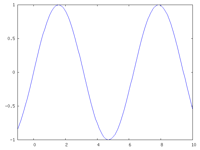
Here x is defined to be an array containing values from -1 to 10, counting by 0.1, i.e. [ -1, -0.9, …, 9.8, 9.9, 10 ]. Then y is set to the array containing the sine of each of these values (it is common for functions to act coordinate-wise in Octave). Finally, the plot is drawn from points with x-coordinates coming from x and y-coordinates coming from y.

Plotting a parameterized curve in Mathematica is as easy as using the ParametricPlot function. For example, to get the plot of a circle,

Plotting a parameterized curve in Maxima is almost as easy as giving a list with both x and y parameters to the Plot2D function. For example, to plot a circle,

To make the plot smoother, specify more ticks.

Plotting a parameterized curve in Axiom is almost as easy as giving ordered pairs with the x and y parameters to the draw() function. For example, to plot a circle,

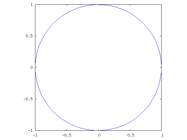
Plotting a parameterized curve in Octave is trivial. In effect, the regular plot() function already gives a plot of a parametrized function. It’s just that using x as the parameter is the most typical use. However, nothing stops us from using it in a more general fashion. For example, to plot a circle:

The circle may appear out of shape if the scales of the axes aren’t drawn the same (resizing the window will correct the shape). You can ask gnuplot to draw the axes with precisely the same scales; "ratio -1" is a special setting for gnuplot that makes sure the y-unit and the x-unit have the same size.

On newer versions of Octave, use this instead:

If you would like to interactively rotate the image, older version of Mathematica first need the RealTime3D system. Newer versions of Mathematica already have interactive image manipulation.

The default setting (i.e. no interactive 3D) can be restored via:

There are many attributes you can manipulate on the plot including contour lines and axis label. See Contour plots with Maxima for details.

In current versions of Maxima, the image can be manipulated interactively with the mouse. If you still have an older version of Maxima for Linux and would like to interactively rotate the image, you can specify mgnuplot to generate the plot.

The same draw() command that does 2D plotting does 3D plotting as well. Simply give a third argument with the bounds for the second variable.

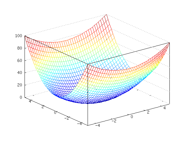
As with 2D plotting, Octave needs a set of points to plot. In this case, there is a function called meshgrid() which can generate them. You pass it an array of the grid-values in the x-direction and the y-direction and it returns two matrices, xx and yy, that contain the coordinates for an entire rectangular grid. Once you have evaluated your function on those points, the mesh() function displays the graph.

The following implementation is equivalent but shorter:

To get a different view use "gset view".

For kicks you might try this animation:

The eval/sprintf construct is required because the parameters passed to gset are not evaluated (so if you put "gset view 45, i" it would complain that "i" was not a number).

We can plot a function like f(x,y) = x^2+y^2 over a general region, like the area enclosed by the curves y=x and y=x^2, by creating a function defined only on our region of interest and plotting that.

We can plot a function like f(x,y) = x^2+y^2 over a general region, like the area enclosed by the curves y=x and y=x^2, by creating a piecewise-defined function (defined to be 0 off our region of interest) and plotting that.

Note: Older versions of Maxima will give an error on this plot. You must tell Maxima not to evaluate the function too early, by enclosing it inside '( ) as in:

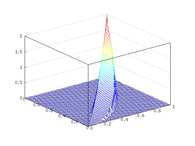
We can plot a function like f(x,y) = x^2+y^2 over a general region, like the area enclosed by the curves y=x and y=x^2, by creating a piecewise-defined function (defined to be 0 off our region of interest) and plotting that.

Newer versions of Maxima can generate contour plots with the contour_plot() function.

Since plotting in Maxima is done by Gnuplot, a contour plot may be manipulated by passing values through to the plotting engine. For example, the number of contour lines may be changed.

Another really dynamic way to visualize contour lines is by drawing them right on a surface. This is also done by passing arguments through to gnuplot, but using the usual plot3d() function.

Perhaps it is easier to see what is happening with the axes labeled. We can easily include that as well.

You may add as many hints to gnuplot as you wish. Gnuplot options/commands you may be interested in trying:

Because Octave uses Gnuplot to display its graphics, it can take advantage of Gnuplot’s ability to create contour lines, just as Maxima can. There is even a pre-built command called contour that automates some of this. It takes as arguments: a matrix of z-values, the number of contours to draw, a vector of x-coordinates, and a vector of y-coordinates.

Notice that the setup is much the same as for 3D graphing, and so you can start from a 3D plot and adjust the rest of the settings in any way you like. Continuing the calculations from above,

Alternative Method

Because Octave is FreeSoftware, we are free to modify it if we wish. For technical reasons, it is awkward that Octave draws contour lines by manipulating a 3D graph object. For one thing, it means that we are not free to draw other 2D objects on the same graph.

To make a real 2D contour plot (on a Linux system) download contour-2.1.tar.gz. This file contains source code for a new contour plot function for Octave 2.1. If you are still running version 2.0, you can use contour.tar.gz. To build it,

When you start Octave from this directory, you now have access to a new contour plot function.

Note that the arguments are are changed from the original. They match the mesh() function. Now a simple variation of the previous directions will generate a beautiful contour plot.

One technical advantage of using this method to draw contour lines is that you can add other 2D drawings to a contour plot. That makes it possible to do things like this exploration lab of the gradient vector: pdf/ps

Plotting a surface together with its tangent plane is a matter of generating two plots and displaying them together with the Show command.

For example, the surface z = x^2 - y^2 at the point (1,2,-3) has the tangent plane z+3 = 2(x-1) -4(x-2). We can verify this by calculating the partial derivatives using Mathematica.

Generate a plot of each function using the Plot3D command. Here, we we use the argument DisplayFunction->Identity because we don’t care to see the individual graphs. We’ll define the surface on a square domain from -3 to 3 but the tangent plane will only exist around the point (1,2,-3). This will make the plane appear as a small flat patch against the surface.

Now we show both plots together, using the Show function. I am uncertain precisely what the DisplayFunction part means, but it is necessary to make the graph appear. Unfortunately, the view is bad, so a custom ViewPoint also helps.

Plotting a surface together with its tangent plane is only a small adaptation of the 3D plotting directions given above. The method is to plot the surface as usual, give the "hold on" command to preserve the surface, and then plot the plane.

For example, the surface z = x^2 - y^2 at the point (1,2,-3) has the tangent plane z+3 = 2(x-1) -4(x-2). To get a view of the surface and tangent together, first plot the surface.

To make it easier to spot the tangent plane, we’ll only define it nearby the point (1,2,-3), not on the entire domain. Notice how below we set a smaller x domain of (0.5,1.5) and a smaller y domain of (1.5,2.5). This will make the tangent plane appear as a small patch against the curved surface.

Here we use "hold on" to keep the surface visible while we add the plane.

Rotate the surface however you like and replot to get a good view:

Perhaps some transparency will help:

The ParametricPlot3D[] function can plot parametric curves and parametric surfaces in 3-space.

When the first argument of plot3d() is a vector, Maxima performs a parametric plot. The vector argument can be a vector-valued function as shown here, or an explicit vector.

Plotting in Octave is simply a matter of generating (x,y,z) coordinates for the mesh() function. If a surface is parametrized by <x,y,z> = <2*(cos(v) + u*cos(v/2)*cos(v)), 2*(sin(v) + u*cos(v/2)*sin(v)), 2*u*sin(v/2)> then this is how it would be drawn in Octave:

In Axiom, a parameterized surface is drawn using the same draw() function as other kinds of plots. It is almost as simple as passing the parametrizations straight through: For <x,y,z> = <2*(cos(v) + u*cos(v/2)*cos(v)), 2*(sin(v) + u*cos(v/2)*sin(v)), 2*u*sin(v/2)> the plot would be:

Say you have z(x,y) = x^2*y + 3*x*y^4 where x = x(t) = sin(2*t) and y = y(t) = cos(t). Then effectively, z is a function of t and we can calculate dz/dt. But what does this mean? Well, the vector <x(t),y(t),z(t)> parametrizes a curve in 3-space, and dz/dt is the slope as you travel around via the paramentrization (as opposed, say, to in the x-direction or y-direction).

We can get a view of this curve using the ParametricPlot3D function of Mathematica.

Say you have z(x,y) = x^2*y + 3*x*y^4 where x = x(t) = sin(2*t) and y = y(t) = cos(t). Then effectively, z is a function of t and we can calculate dz/dt. But what does this mean? Well, the vector <x(t),y(t),z(t)> parametrizes a curve in 3-space, and dz/dt is the slope as you travel around via the paramentrization (as opposed, say, to in the x-direction or y-direction).

So, how can we get a view of this curve? We use the parametric plotting capability of Maxima, by giving a list of functions [x,y,z] as the argument to plot. We also have to cheat a bit. Maxima expects two domain variables to be defined. So we define a real variable t and a dummy variable u, which we never use. For efficiency, we can declare the number of grid points to use for each variable, and we condemn u to use only 1.

Say you have z(x,y) = x^2*y + 3*x*y^4 where x = x(t) = sin(2*t) and y = y(t) = cos(t). Then effectively, z is a function of t and we can calculate dz/dt. But what does this mean? Well, the vector <x(t),y(t),z(t)> parametrizes a curve in 3-space, and dz/dt is the slope as you travel around via the paramentrization (as opposed, say, to in the x-direction or y-direction).

So, how can we get a view of this curve? Essentially, you need only get the (x,y,z) coordinates together and the mesh() function can plot it. First the functions need to be defined.

There’s only one catch after that. The mesh() function behaves differently when it receives vectors for arguments than when it receives matrices. We really want the matrix behavior, so we’ll double the (single) row of a vector of time values t and call the matrix tt. That will ensure that xx, yy, and zz defined from it are all matrices with two rows. Essentially, we’ll ask Octave to plot the curve twice, but no harm comes from doing that.

From tt, we define all of the points of the parametrized curve and plot them with mesh().

Finally, the graph may be rotated like any other 3D graph. For example, borrowing an idea from above:

You have to load Graphics`PlotField` before you create vector field plots. After that, to plot the vector field F(x,y) = <1,-1> on the domain [0,10]x[0,10],

To plot the vector field F(x,y) = <-y,x> on [-3,3]x[-3,3],

You have to load draw before you create vector field plots, and you’ll also need to create a quiver function.

After that, to plot the vector field F(x,y) = <1,-1> on the domain [0,10]x[0,10], you call the quiver function with the components (defined in terms of x and y) and coordinate ranges. The last argument controls scaling. If it is 0, you’ll get an unscaled plot, but this is sometimes visually overwhelming. If you pass a 1, the vectors will be auto-scaled to prevent overlapping. You can use numbers larger or smaller than 1 to stretch and shrink the auto-scaled arrows.

To plot the vector field F(x,y) = <-y,x> on [-3,3]x[-2,2],

Alternate solution: If you prefer Mathematica-like syntax, then load the draw module, and use the following plot_vector_field function:

After that, to plot the vector field F(x,y) = <1,-1> on the domain [0,10]x[0,10], you call the plot_vector_field function with the vector function and coordinate ranges. The last argument controls scaling. If it is 0, you’ll get an unscaled plot, but this is sometimes visually overwhelming. If you pass a 1, the vectors will be auto-scaled to prevent overlapping. You can use numbers larger or smaller than 1 to stretch and shrink the auto-scaled arrows.

To plot the vector field F(x,y) = <-y,x> on [-3,3]x[-2,2],

Using the small m-file quiver.m (save it in your working directory before you start octave), you can create 2D plots of vector fields. The quiver function accepts 4 arguments, (x,y) coordinates of the domain of the vector field, and the (u,v) coordinates of the vectors.

For example, to plot the vector field F(x,y) = <1,-1> on the domain [0,10]x[0,10],

To plot the vector field F(x,y) = <-y,x> on [-3,3]x[-3,3],

You have to load Graphics`PlotField3D` before you create 3D vector field plots. You’ll probably also want to load RealTime3D` so you can interactively rotate your plots (static 3D vector field plots can be difficult to decipher).

To plot the vectorfield F(x,y,z) = <-y,x,z>,

You have to load draw before you create vector field plots, and you’ll also need to create a quiver3 function.

After that, to plot the vector field F(x,y,z) = <-y,x,z> on the domain [-2,2]x[-3,3]x[-4,4], you call the quiver3 function with the components (defined in terms of x,y,and z) and coordinate ranges. The last argument controls scaling. If it is 0, you’ll get an unscaled plot, but this is sometimes visually overwhelming. If you pass a 1, the vectors will be auto-scaled to prevent overlapping. You can use numbers larger or smaller than 1 to stretch and shrink the auto-scaled arrows.

Alternate solution: If you prefer Mathematica-like syntax, then load the draw module, and use the following plot_vector_field3d function:

After that, to plot the vector field F(x,y,z) = <-y,x,z> on the domain [-2,2]x[-3,3]x[-4,4], you call the plot_vector_field3d function with the vector function and coordinate ranges. The last argument controls scaling. If it is 0, you’ll get an unscaled plot, but this is sometimes visually overwhelming. If you pass a 1, the vectors will be auto-scaled to prevent overlapping. You can use numbers larger or smaller than 1 to stretch and shrink the auto-scaled arrows.

Octave (as it is installed on ice) doesn’t quite have what it needs to do plots of 3D vector fields. The most important thing that is missing is a newer version of gnuplot. I’ve installed the development version of gnuplot in my home account. You can tell octave to use it by editing your .octaverc file and inserting the following line.

The second thing you’ll need is an updated meshgrid() function, which can generate 3D meshgrids. I have one in meshgrid.m (save a copy in your working directory to use it). Then, using the small m-file quiver3.m, you can create 3D plots of vector fields. The quiver3() function accepts 6 arguments, (x,y,z) coordinates of the domain of the vector field, and the (u,v,w) coordinates of the vectors.

To plot the vectorfield F(x,y,z) = <-y,x,z>,

Even with the help of a computer, 3D vector fields can be hard to visualize. Often the arrows are long and overlapping. So quiver3() automatically scales the arrows. Add an optional argument to turn off autoscaling (0) or to adjust the arrow length. Set it to a value between 0 and 1 to shorten the arrows or to a value greater than 1 to lengthen them.

Maxima doesn’t have a commmand for printing a plot, but it does have options for saving a plot to a file, which you can then print. The most useful file formats are probably Postscript and png (and perhaps dumb, which saves your plot as ASCII art). Since maxima uses gnuplot for its plotting, we simply have Maxima tell gnuplot how to handle our plot.

The first command here saves our plot as a Postscript file called maxplot.ps and the second saves a png file maxplot.png:

We can also specify a file name if we wish: